
 Software Tutorial
Office Software
Rotate charts in Excel - spin bar, column, pie and line charts
Software Tutorial
Office Software
Rotate charts in Excel - spin bar, column, pie and line charts
Rotate charts in Excel - spin bar, column, pie and line charts
May 19, 2025 am 09:44 AM
This article will guide you how to rotate a chart in Excel. You'll learn how to rotate bar charts, bar charts, pie charts, and line charts, including their 3D variants. Additionally, you will learn how to reverse the drawing order of values, categories, series, and legends. For users who frequently print charts, this article will also introduce how to adjust the printing direction of a worksheet.
Excel makes it very easy to represent table data as a chart or graph. You just select the data and click on the appropriate chart type icon. However, the default settings may not meet your needs. If your task is to rotate a chart in Excel to rearrange slices, bars, bars, or line charts of a pie chart, this article will help you.
### Rotate pie charts to any angle you like in ExcelIf you often deal with relative sizes and show overall scale, you might use a pie chart. In the image below, the data label overlaps with the title, making it look unsightly. I'm going to copy it into my PowerPoint presentation about people's eating habits and want the chart to look neat and orderly. To solve this problem and highlight the most important facts, you need to know how to rotate a pie chart clockwise in Excel.

Right-click any slice of the pie chart and select the Format Data Series… option from the menu.

-
You will see the Format Data Series pane. Go to the angle box of the first slice , enter the number of angles you need (rather than 0), and press Enter . I think 190 degrees fit my pie chart.
My Excel pie chart after the spin looks neat and orderly.


So, you can see that it is very simple to rotate the Excel chart to any angle to achieve the effect you need. This is very helpful for fine-tuning the label layout or highlighting the most important slices.
Rotate 3D Charts in Excel: Rotate Pie Charts, Bar Charts, Line Charts and Bar Charts
I think 3D charts look great. When others see your 3D charts, they may think you know everything about Excel visualization. If the chart created with the default settings does not meet your needs, you can adjust it by rotating and changing the perspective.

Right-click on your chart and select 3D Rotation from the menu list… .
-
You will see the Format Chart Area pane with all the settings available. Enter the necessary number of angles in the X and Y rotation boxes.
I changed the numbers to 40 and 35 to make my chart look slightly deeper.


This pane also allows you to adjust depth and height , as well as perspective . Just play around with these options and see which chart types are best for you. You can also use the same steps for pie charts.
Rotate the chart by 180 degrees: Change the order of categories, values, or series
If you need to rotate the Excel chart to display horizontal and vertical axes, you can quickly reverse the order of categories or numeric values ??drawn along those axes. Additionally, in a 3D chart with depth axes, you can flip the drawing order of the data series so that the large 3D columns do not obstruct smaller columns. You can also reposition the legend in Excel's pie chart or bar chart.
Reverse the drawing order of categories in the chart
You can rotate your chart based on the horizontal (category) axis .

- Right-click on the horizontal axis and select the Format Axis… option from the menu.
- You will see the Format Axis pane. Simply check the checkbox next to the category order invert to see your chart rotate 180 degrees.


Reverse the drawing order of values ??in the chart
Follow the following simple steps to rotate the values ??on the vertical axis.

Right-click the vertical (value) axis and select the Format Axis… option.
-
Select the Invert Numeric Order check box.
Note: Remember that the drawing order of values ??cannot be reversed in the radar graph.


Reverse the drawing order of data series in 3D charts
If you have a bar or line chart with a third axis that shows some columns (lines) in front of others (lines), you can change the order in which the data series is drawn so that the large 3D data markers do not overlap smaller data markers. You can also use the following steps to create two or more charts to display all values ??in the legend.

- Right-click on the Depth (Series) axis on the chart and select the Format Axis… menu item.
- You will see the Format Axis pane open. Check the Invert Series Order check box to see the columns or lines flip.


Change the position of the legend in the chart
In the Excel pie chart below, the legend is at the bottom. I want to move the legend values ??to the right to make them more eye-catching.

Right-click the legend and select the Format Legend… option.
-
In the Legend Options pane, select one of the check boxes you see: top, bottom, left, right , or top right .
Now I prefer my chart.


Modify worksheet orientation to better adapt to your chart
If you just need to print the chart, you might just need to modify the worksheet layout without having to rotate the chart in Excel. In my screenshot below, you can see that the chart is not adapting correctly. By default, the worksheet is printed in portrait (higher than width). I'm changing the layout to landscape mode so that my images look correct on the printable version.

Select a worksheet containing the chart to print.
-
Go to the Page Layout tab and click the arrow under the direction icon. Select the landscape option.
Now when I enter the print preview window, I can see my chart adapting perfectly.


Use the Camera Tool to rotate your Excel chart to any angle
You can rotate the chart to any angle using the Camera tool in Excel. It allows you to place the results next to the original chart or insert them into a new worksheet.
Tip: If you want to rotate the chart 90 degrees, it is a good idea to modify the chart type. For example, change from a bar chart to a bar chart.
You can add the camera tool by going to the Quick Access Toolbar and clicking the small drop-down arrow. Select More Commands… options.

Add the camera by selecting the camera from the list of all commands and clicking Add .

Now follow the steps below to make the camera options work for you.
Note: Remember, you cannot put the camera tool on your chart because the results are unpredictable.
Create your line chart or any other chart.
You may need to flip the alignment of the chart axes to 270 degrees using the format axis option I described above. Therefore, the rotated chart label will be readable.
Select the range of cells that contain the chart.
Click the Camera icon on the Quick Access toolbar .
Click any cell in the table to create a camera object.
Now grab the top rotation control.
-
Rotate your Excel chart to the desired angle and drop the controls.
Note: There is a problem with using the camera tool. The generated objects may be at a lower resolution than the actual chart. They may appear blurry or pixelated.


Creating charts is an excellent way to show your data. Charts in Excel are easy to use, comprehensive, visual, and can be adjusted to the look you need. Now you know how to rotate your bar chart, bar chart, pie chart, or line chart.
After writing the above, I feel like I am really a chart spinner. Hope my article will help you with your tasks as well. I wish you a happy and outstanding performance in Excel!
The above is the detailed content of Rotate charts in Excel - spin bar, column, pie and line charts. For more information, please follow other related articles on the PHP Chinese website!

Hot AI Tools

Undress AI Tool
Undress images for free

Undresser.AI Undress
AI-powered app for creating realistic nude photos

AI Clothes Remover
Online AI tool for removing clothes from photos.

Clothoff.io
AI clothes remover

Video Face Swap
Swap faces in any video effortlessly with our completely free AI face swap tool!

Hot Article
Hot Tools

Notepad++7.3.1
Easy-to-use and free code editor

SublimeText3 Chinese version
Chinese version, very easy to use

Zend Studio 13.0.1
Powerful PHP integrated development environment

Dreamweaver CS6
Visual web development tools

SublimeText3 Mac version
God-level code editing software (SublimeText3)
Hot Topics


 How to Use Parentheses, Square Brackets, and Curly Braces in Microsoft Excel
Jun 19, 2025 am 03:03 AM
How to Use Parentheses, Square Brackets, and Curly Braces in Microsoft Excel
Jun 19, 2025 am 03:03 AM
Quick Links Parentheses: Controlling the Order of Opera
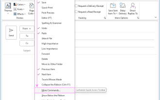 Outlook Quick Access Toolbar: customize, move, hide and show
Jun 18, 2025 am 11:01 AM
Outlook Quick Access Toolbar: customize, move, hide and show
Jun 18, 2025 am 11:01 AM
This guide will walk you through how to customize, move, hide, and show the Quick Access Toolbar, helping you shape your Outlook workspace to fit your daily routine and preferences. The Quick Access Toolbar in Microsoft Outlook is a usefu
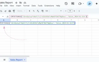 Google Sheets IMPORTRANGE: The Complete Guide
Jun 18, 2025 am 09:54 AM
Google Sheets IMPORTRANGE: The Complete Guide
Jun 18, 2025 am 09:54 AM
Ever played the "just one quick copy-paste" game with Google Sheets... and lost an hour of your life? What starts as a simple data transfer quickly snowballs into a nightmare when working with dynamic information. Those "quick fixes&qu
 Don't Ignore the Power of F9 in Microsoft Excel
Jun 21, 2025 am 06:23 AM
Don't Ignore the Power of F9 in Microsoft Excel
Jun 21, 2025 am 06:23 AM
Quick LinksRecalculating Formulas in Manual Calculation ModeDebugging Complex FormulasMinimizing the Excel WindowMicrosoft Excel has so many keyboard shortcuts that it can sometimes be difficult to remember the most useful. One of the most overlooked
 6 Cool Right-Click Tricks in Microsoft Excel
Jun 24, 2025 am 12:55 AM
6 Cool Right-Click Tricks in Microsoft Excel
Jun 24, 2025 am 12:55 AM
Quick Links Copy, Move, and Link Cell Elements
 Prove Your Real-World Microsoft Excel Skills With the How-To Geek Test (Advanced)
Jun 17, 2025 pm 02:44 PM
Prove Your Real-World Microsoft Excel Skills With the How-To Geek Test (Advanced)
Jun 17, 2025 pm 02:44 PM
Whether you've recently taken a Microsoft Excel course or you want to verify that your knowledge of the program is current, try out the How-To Geek Advanced Excel Test and find out how well you do!This is the third in a three-part series. The first i
 How to recover unsaved Word document
Jun 27, 2025 am 11:36 AM
How to recover unsaved Word document
Jun 27, 2025 am 11:36 AM
1. Check the automatic recovery folder, open "Recover Unsaved Documents" in Word or enter the C:\Users\Users\Username\AppData\Roaming\Microsoft\Word path to find the .asd ending file; 2. Find temporary files or use OneDrive historical version, enter ~$ file name.docx in the original directory to see if it exists or log in to OneDrive to view the version history; 3. Use Windows' "Previous Versions" function or third-party tools such as Recuva and EaseUS to scan and restore and completely delete files. The above methods can improve the recovery success rate, but you need to operate as soon as possible and avoid writing new data. Automatic saving, regular saving or cloud use should be enabled
 5 New Microsoft Excel Features to Try in July 2025
Jul 02, 2025 am 03:02 AM
5 New Microsoft Excel Features to Try in July 2025
Jul 02, 2025 am 03:02 AM
Quick Links Let Copilot Determine Which Table to Manipu
