

How to set excel to hide numbers after removing decimal point
May 10, 2021 pm 02:13 PM
How to hide numbers after removing decimal points in excel: First select the data area and right-click; then select the format cell option in the pop-up options; finally select the value and set the number of decimal points to 0. Just click OK.

The operating environment of this article: windows10 system, microsoft office excel 2010, thinkpad t480 computer.
The specific steps are as follows:
First select the required data area, then right-click the mouse and select the Format Cells button.

Select the numerical option on the left.

Set the number of decimal points to "0", and then click the OK button, so that Excel will remove the numbers hidden after the decimal point.

Related recommendations: windows system
The above is the detailed content of How to set excel to hide numbers after removing decimal point. For more information, please follow other related articles on the PHP Chinese website!

Hot AI Tools

Undress AI Tool
Undress images for free

Undresser.AI Undress
AI-powered app for creating realistic nude photos

AI Clothes Remover
Online AI tool for removing clothes from photos.

Clothoff.io
AI clothes remover

Video Face Swap
Swap faces in any video effortlessly with our completely free AI face swap tool!

Hot Article
Hot Tools

Notepad++7.3.1
Easy-to-use and free code editor

SublimeText3 Chinese version
Chinese version, very easy to use

Zend Studio 13.0.1
Powerful PHP integrated development environment

Dreamweaver CS6
Visual web development tools

SublimeText3 Mac version
God-level code editing software (SublimeText3)


 What should I do if the frame line disappears when printing in Excel?
Mar 21, 2024 am 09:50 AM
What should I do if the frame line disappears when printing in Excel?
Mar 21, 2024 am 09:50 AM
If when opening a file that needs to be printed, we will find that the table frame line has disappeared for some reason in the print preview. When encountering such a situation, we must deal with it in time. If this also appears in your print file If you have questions like this, then join the editor to learn the following course: What should I do if the frame line disappears when printing a table in Excel? 1. Open a file that needs to be printed, as shown in the figure below. 2. Select all required content areas, as shown in the figure below. 3. Right-click the mouse and select the "Format Cells" option, as shown in the figure below. 4. Click the “Border” option at the top of the window, as shown in the figure below. 5. Select the thin solid line pattern in the line style on the left, as shown in the figure below. 6. Select "Outer Border"
 How to filter more than 3 keywords at the same time in excel
Mar 21, 2024 pm 03:16 PM
How to filter more than 3 keywords at the same time in excel
Mar 21, 2024 pm 03:16 PM
Excel is often used to process data in daily office work, and it is often necessary to use the "filter" function. When we choose to perform "filtering" in Excel, we can only filter up to two conditions for the same column. So, do you know how to filter more than 3 keywords at the same time in Excel? Next, let me demonstrate it to you. The first method is to gradually add the conditions to the filter. If you want to filter out three qualifying details at the same time, you first need to filter out one of them step by step. At the beginning, you can first filter out employees with the surname "Wang" based on the conditions. Then click [OK], and then check [Add current selection to filter] in the filter results. The steps are as follows. Similarly, perform filtering separately again
 How to read excel data in html
Mar 27, 2024 pm 05:11 PM
How to read excel data in html
Mar 27, 2024 pm 05:11 PM
How to read excel data in html: 1. Use JavaScript library to read Excel data; 2. Use server-side programming language to read Excel data.
 How to insert excel icons into PPT slides
Mar 26, 2024 pm 05:40 PM
How to insert excel icons into PPT slides
Mar 26, 2024 pm 05:40 PM
1. Open the PPT and turn the page to the page where you need to insert the excel icon. Click the Insert tab. 2. Click [Object]. 3. The following dialog box will pop up. 4. Click [Create from file] and click [Browse]. 5. Select the excel table to be inserted. 6. Click OK and the following page will pop up. 7. Check [Show as icon]. 8. Click OK.
 Get data from Excel via HTML: A comprehensive guide
Apr 09, 2024 am 10:03 AM
Get data from Excel via HTML: A comprehensive guide
Apr 09, 2024 am 10:03 AM
How to get Excel data in HTML? Import Excel files: using elements. Parse Excel files: use xlsx library or browser functionality. Get data: Get the worksheet object, including row and column data. Display data: Use HTML elements (such as tables) to display data.
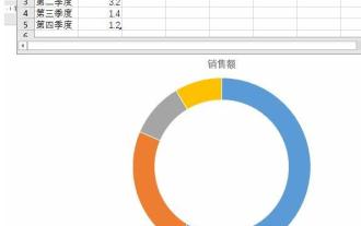 Detailed method of inserting Excel circular data chart into PPT
Mar 26, 2024 pm 04:26 PM
Detailed method of inserting Excel circular data chart into PPT
Mar 26, 2024 pm 04:26 PM
1. Create a new PPT page and insert the Excel ring chart. 2. Delete the redundant data in the table, leaving two rows of data, and set them in percentage form to facilitate parameter setting. 3. Copy the data in column B to other columns according to display needs. From the sample picture of this column, you can see what it looks like when copying 5 columns. Pay attention to why the animation operation does not use dragging cells to copy, but the honest and practical method of copying and pasting. You will experience it when you actually operate it. 4. After copying N pieces, set the orange part to no color, and you are done. Note: 1. Use PPT to make information charts like this, which can be drawn graphically or accurately produced using Excel data. 2. This technique is valid for Excel 2007 and above.
 Complete collection of excel function formulas
May 07, 2024 pm 12:04 PM
Complete collection of excel function formulas
May 07, 2024 pm 12:04 PM
1. The SUM function is used to sum the numbers in a column or a group of cells, for example: =SUM(A1:J10). 2. The AVERAGE function is used to calculate the average of the numbers in a column or a group of cells, for example: =AVERAGE(A1:A10). 3. COUNT function, used to count the number of numbers or text in a column or a group of cells, for example: =COUNT(A1:A10) 4. IF function, used to make logical judgments based on specified conditions and return the corresponding result.
 How to copy a table in Excel and keep the original format?
Mar 21, 2024 am 10:26 AM
How to copy a table in Excel and keep the original format?
Mar 21, 2024 am 10:26 AM
We often use Excel to process multiple table data. After copying and pasting the set table, the original format returns to the default, and we have to reset it. In fact, there is a way to make the Excel copy table retain the original format. The editor will explain the specific method to you below. 1. Ctrl key dragging and copying operation steps: Use the shortcut key [Ctrl+A] to select all table contents, then move the mouse cursor to the edge of the table until the moving cursor appears. Press and hold the [Ctrl] key, and then drag the table to the desired position to complete the movement. It should be noted that this method only works on a single worksheet and cannot be moved between different worksheets. 2. Steps for selective pasting: Press the [Ctrl+A] shortcut key to select all tables, and press
