
 Software Tutorial
Office Software
The Ultimate Guide to Define Formula in Excel: Functions and Examples
Software Tutorial
Office Software
The Ultimate Guide to Define Formula in Excel: Functions and Examples
The Ultimate Guide to Define Formula in Excel: Functions and Examples
May 16, 2025 pm 05:47 PM
Excel is celebrated for its robust capabilities in managing both simple and complex data operations. Central to Excel's versatility are formulas and functions, which are crucial tools for users looking to optimize their calculations and data manipulation. This article aims to unravel these components, providing insights into their application and illustrating practical examples. Whether you are a beginner or seeking to refine your skills, mastering Excel formulas will undoubtedly boost your productivity.
Key Takeaways:
- Excel formulas facilitate automated calculations and dynamically update when data changes.
- Fundamental functions such as SUM, AVERAGE, and COUNT streamline data analysis.
- IF and VLOOKUP functions enhance spreadsheets with logic and lookup capabilities.
- INDEX-MATCH offers a versatile and efficient alternative to VLOOKUP for data retrieval.
- Understanding common errors like #DIV/0! and #VALUE! ensures the accuracy of your spreadsheets.
Table of Contents
Unraveling Excel Formulas
What is a Formula in Excel?
In Excel, a formula is an expression that conducts calculations on cell values. Formulas can range from simple additions to complex analyses of large datasets. Their power lies in their ability to automatically update whenever the data in referenced cells changes.
Every formula in Excel starts with an equal sign (=), followed by a mix of numbers, cell references, functions, and operators. For example, to add two numbers in Excel, you could type:
=5 3

This formula will yield 8.
Essential Excel Functions You Should Know
SUM, AVERAGE, and COUNT Functions
The SUM, AVERAGE, and COUNT functions are foundational tools in Excel, offering efficient methods for performing basic arithmetic and counting data. They are vital for users looking to quickly process and analyze datasets.
- SUM Function: This function sums up all the specified values, making it indispensable for calculating totals across rows or columns. For instance, =SUM(A2:A10) calculates the sum of the values in cells A2 through A10.

- AVERAGE Function: It computes the mean of a range, providing insights into the central tendency of data. Using =AVERAGE(A2:A10), you can find the average, which is useful for trend analysis or comparing datasets over time.

- COUNT Function: This function counts the number of cells with numerical data within a specified range. It's especially useful for quantifying entries or understanding data volume—simply use =COUNT(A2:A10) to count the numerical entries in that range.

These functions automate crucial calculations, thereby enhancing data analysis and helping users extract meaningful insights from their data.
IF and VLOOKUP Functions Explained
The IF and VLOOKUP functions are powerful tools in Excel that add logic and lookup capabilities to your spreadsheets, significantly expanding the potential for data manipulation and analysis.
- IF Function: The IF function introduces conditional logic into your spreadsheets. It performs one of two actions based on a condition, making it perfect for scenarios that require simple conditional operations. Its syntax, =IF(condition, value_if_true, value_if_false), allows actions such as =IF(A1>50, "Pass", "Fail"), where the cell's value determines whether a student passes or fails.

- VLOOKUP Function: VLOOKUP, or Vertical Lookup, searches for a value in the first column of a table and returns a related value from a specified column. It simplifies data retrieval, particularly in large databases, by matching entries. For example, using =VLOOKUP(105, A2:C10, 2, FALSE) locates the value corresponding to '105' in the first column and retrieves associated data from the second column, aiding tasks like tracking financial records or inventory items.

Together, IF and VLOOKUP provide dynamic methods to tailor calculations and extract meaningful data, enabling users to perform complex decision-making and data management with precision.
Exploring the Power of INDEX-MATCH
The INDEX-MATCH combination is a powerful duo in Excel, offering a more flexible and efficient alternative to the traditional VLOOKUP function. They provide a robust method for data retrieval, especially when dealing with large and dynamic datasets.
- INDEX Function: This function retrieves a value or reference from within an array or table, based on specified row and column numbers. Its syntax is =INDEX(array, row_num, [column_num]), allowing for precise data extraction. For instance, =INDEX(A2:B10,5,2) retrieves data from the third row and second column of the specified array.

- MATCH Function: The MATCH function complements INDEX by identifying the position of a specific value within a range. The syntax =MATCH(lookup_value, lookup_array, [match_type]) offers flexibility in finding exact or approximate matches, such as locating the position of "Smith" in a column.

- Combining INDEX and MATCH: When used together, INDEX-MATCH offers a robust solution for data lookup. Unlike VLOOKUP, which requires the lookup column to be the first one, INDEX-MATCH allows searching any column in the table array, enhancing versatility and efficiency. For example, =INDEX(A2:B10,MATCH(105,A2:A10,0),2) finds and returns the score associated with "105" by searching in a different column, thus highlighting its capability to navigate complex data structures.

This combination also outperforms VLOOKUP in terms of performance, as it requires less processing power by focusing only on relevant columns. Hence, INDEX-MATCH is preferred for tasks requiring precision and adaptability, such as financial modeling and detailed reporting, making it essential for advanced Excel users.
Common Errors and Their Solutions
Troubleshooting #DIV/0!, #VALUE!, and Other Errors
Excel errors like #DIV/0! and #VALUE! can interrupt your workflow if not addressed promptly. Understanding their causes and solutions is key to maintaining efficient and accurate spreadsheets.
#DIV/0! Error: This error occurs when a formula attempts to divide a number by zero or an empty cell. To resolve it, ensure that divisors are non-zero and that cells referenced in calculations contain valid data. Using the IFERROR function, such as =IFERROR(A2/B2, "Error"), can handle the error gracefully by displaying "Error" if a division by zero is attempted.

#VALUE! Error: This error typically arises when a formula uses incorrect data types, such as attempting arithmetic on text values. Verify that all cell references point to numerical values and ensure correct data input throughout your spreadsheet. Resolving this often involves converting cell content to appropriate numerical data or using functions to convert text to numbers.

Other Common Errors: Errors like #REF! occur when a formula refers to a cell that no longer exists, typically due to deletion. Check cell references for accuracy and update them as needed.

The #NAME? error indicates a misspelled function or range name—ensure all formula components are correctly spelled and exist within the workbook.

To effectively troubleshoot and resolve these errors:
- Double-Check References: Ensure all cell references are accurate and point to the intended data ranges.
- Verify Data Types: Make sure the data used in formulas is in the correct format (numbers for calculations, text for specific functions).
- Utilize Built-in Tools: Excel’s ‘Error Checking’ tool can be invaluable in diagnosing and addressing formula errors.
Understanding these errors and applying appropriate solutions not only maintains the integrity of your data but also enhances the overall functionality of your Excel sheets, enabling seamless and efficient data analysis.
FAQs
How to define a function in Excel?
To define a function in Excel, select an empty cell where you want the result, type an equal sign (=), and then enter the function name followed by its arguments within parentheses. For example, to calculate the sum of sales, use =SUM(A1:A10), specifying the cell range to include in the operation.
What are the basic differences between formulas and functions in Excel?
Formulas are user-defined equations for calculations, combining operators and cell references (e.g., =A1 B1). Functions are predefined in Excel, executing specific tasks with given arguments (e.g., SUM or AVERAGE). While functions simplify complex calculations, formulas offer customization.
How can I apply a formula to an entire column?
To apply a formula to an entire column in Excel, select the cell containing the formula and use the fill handle by dragging it down the column. Alternatively, press CTRL D to fill down if you’ve selected the formula cell and the cells below it. You can also double-click the fill handle to quickly apply the formula to all adjacent cells in the column.
Can Excel handle large datasets with complex formulas?
Yes, Excel can handle large datasets with complex formulas. It efficiently processes calculations on thousands of rows. However, performance may vary depending on your system’s capabilities, and for extremely large datasets, optimizing formulas and using Excel’s built-in features like PivotTables can improve efficiency.
The above is the detailed content of The Ultimate Guide to Define Formula in Excel: Functions and Examples. For more information, please follow other related articles on the PHP Chinese website!

Hot AI Tools

Undress AI Tool
Undress images for free

Undresser.AI Undress
AI-powered app for creating realistic nude photos

AI Clothes Remover
Online AI tool for removing clothes from photos.

Clothoff.io
AI clothes remover

Video Face Swap
Swap faces in any video effortlessly with our completely free AI face swap tool!

Hot Article
Hot Tools

Notepad++7.3.1
Easy-to-use and free code editor

SublimeText3 Chinese version
Chinese version, very easy to use

Zend Studio 13.0.1
Powerful PHP integrated development environment

Dreamweaver CS6
Visual web development tools

SublimeText3 Mac version
God-level code editing software (SublimeText3)
Hot Topics


 How to Use Parentheses, Square Brackets, and Curly Braces in Microsoft Excel
Jun 19, 2025 am 03:03 AM
How to Use Parentheses, Square Brackets, and Curly Braces in Microsoft Excel
Jun 19, 2025 am 03:03 AM
Quick Links Parentheses: Controlling the Order of Opera
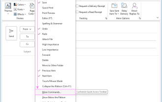 Outlook Quick Access Toolbar: customize, move, hide and show
Jun 18, 2025 am 11:01 AM
Outlook Quick Access Toolbar: customize, move, hide and show
Jun 18, 2025 am 11:01 AM
This guide will walk you through how to customize, move, hide, and show the Quick Access Toolbar, helping you shape your Outlook workspace to fit your daily routine and preferences. The Quick Access Toolbar in Microsoft Outlook is a usefu
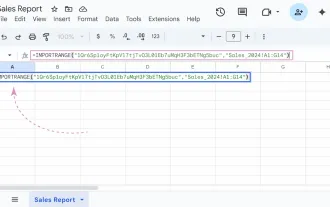 Google Sheets IMPORTRANGE: The Complete Guide
Jun 18, 2025 am 09:54 AM
Google Sheets IMPORTRANGE: The Complete Guide
Jun 18, 2025 am 09:54 AM
Ever played the "just one quick copy-paste" game with Google Sheets... and lost an hour of your life? What starts as a simple data transfer quickly snowballs into a nightmare when working with dynamic information. Those "quick fixes&qu
 6 Cool Right-Click Tricks in Microsoft Excel
Jun 24, 2025 am 12:55 AM
6 Cool Right-Click Tricks in Microsoft Excel
Jun 24, 2025 am 12:55 AM
Quick Links Copy, Move, and Link Cell Elements
 Don't Ignore the Power of F9 in Microsoft Excel
Jun 21, 2025 am 06:23 AM
Don't Ignore the Power of F9 in Microsoft Excel
Jun 21, 2025 am 06:23 AM
Quick LinksRecalculating Formulas in Manual Calculation ModeDebugging Complex FormulasMinimizing the Excel WindowMicrosoft Excel has so many keyboard shortcuts that it can sometimes be difficult to remember the most useful. One of the most overlooked
 Prove Your Real-World Microsoft Excel Skills With the How-To Geek Test (Advanced)
Jun 17, 2025 pm 02:44 PM
Prove Your Real-World Microsoft Excel Skills With the How-To Geek Test (Advanced)
Jun 17, 2025 pm 02:44 PM
Whether you've recently taken a Microsoft Excel course or you want to verify that your knowledge of the program is current, try out the How-To Geek Advanced Excel Test and find out how well you do!This is the third in a three-part series. The first i
 How to recover unsaved Word document
Jun 27, 2025 am 11:36 AM
How to recover unsaved Word document
Jun 27, 2025 am 11:36 AM
1. Check the automatic recovery folder, open "Recover Unsaved Documents" in Word or enter the C:\Users\Users\Username\AppData\Roaming\Microsoft\Word path to find the .asd ending file; 2. Find temporary files or use OneDrive historical version, enter ~$ file name.docx in the original directory to see if it exists or log in to OneDrive to view the version history; 3. Use Windows' "Previous Versions" function or third-party tools such as Recuva and EaseUS to scan and restore and completely delete files. The above methods can improve the recovery success rate, but you need to operate as soon as possible and avoid writing new data. Automatic saving, regular saving or cloud use should be enabled
 5 New Microsoft Excel Features to Try in July 2025
Jul 02, 2025 am 03:02 AM
5 New Microsoft Excel Features to Try in July 2025
Jul 02, 2025 am 03:02 AM
Quick Links Let Copilot Determine Which Table to Manipu
