


This tutorial shows how to use INDEX and MATCH functions in Excel and why it is better than VLOOKUP.
In recent articles, we strive to explain the basics of VLOOKUP functions to beginners and provide more complex examples of VLOOKUP formulas for advanced users. Now, I'll try not just to persuade you not to use VLOOKUP, but to at least show an alternative to doing vertical lookups in Excel.
"Why do I need this?" you might ask. Because VLOOKUP has many limitations, it may prevent you from getting the desired result in many cases. On the other hand, the INDEX MATCH combination is more flexible and has many excellent features that make it superior to VLOOKUP in many ways.

Since the purpose of this tutorial is to show how to perform alternative vertical lookups in Excel by combining INDEX and MATCH functions, we will not discuss their syntax and usage in detail. We will only cover the minimum required to understand the overarching concept and then dive into formula examples that reveal all the advantages of using INDEX MATCH instead of VLOOKUP.
INDEX functions - Syntax and usage
Excel's INDEX function returns a value from the array based on the row and column numbers you specified. The syntax of the INDEX function is very simple:
INDEX(array, row_num, [column_num]) The following is a simple explanation of each parameter:
- array - range of cells from which you want to return the value.
- row_num - The row number in the array from which you want to return the value. If omitted, column_num is required.
- column_num - The column number in the array from which you want to return the value. If omitted, row_num is required.
For more information, see Excel INDEX functions.
Here is the simplest example of INDEX formula:
=INDEX(A1:C10,2,3)
This formula searches cells A1 to C10 and returns the cell value of row 2 and column 3, i.e. cell C2.
Very simple, right? However, when you process real data, you almost never know the row and column numbers you want, which is where the MATCH function comes in handy.
MATCH function - Syntax and usage
Excel's MATCH function searches for a value within a range of cells and returns the relative position of the value in the range.
The syntax of the MATCH function is as follows:
MATCH(lookup_value, lookup_array, [match_type]) - lookup_value - the number or text value you are looking for.
- lookup_array - range of cells being searched for.
- match_type - Specifies whether to return an exact match or the closest match:
- 1 or omit (default) - Approximate match (next smaller).
- 0 - Exact match. In the INDEX/MATCH combination you almost always need an exact match, so you set the third parameter of the MATCH function to 0.
- -1 - Approximate match (next larger).
For example, if range B1:B3 contains the values ??"New-York", "Paris", "London", the following formula returns the number 3, because "London" is the third entry in the range:
=MATCH("London",B1:B3,0)
For more information, see Excel MATCH functions.
At first glance, the use of the MATCH function seems to be questionable. Who cares about the position of the value in the range? What we really want to know is the value itself.
Let me remind you that the relative position of the search value (i.e. row and column number) is exactly what you need to provide to the row_num and column_num parameters to the INDEX function. You remember that Excel INDEX can find the value at the intersection of a given row and column, but it cannot determine the specific row and column you want.
How to use INDEX MATCH function in Excel
Now that you have learned the basics, I believe you have begun to understand how MATCH and INDEX work together. In short, INDEX finds values ??through column and row number lookups, while MATCH provides these numbers. That's it!
For vertical lookup, you only use the MATCH function to determine the row number and directly provide the column range to INDEX:
INDEX ( column from which the value is to be returned , MATCH ( column to be found , 0)) is still difficult to understand? It may be easier to understand by means of an example. Suppose you have a list of national capitals and their populations:

To find the population of a capital, such as the capital of Japan, use the following INDEX MATCH formula:
=INDEX(C2:C10, MATCH("Japan", A2:A10, 0))
Now, let's analyze what each component of this formula actually does:
- The MATCH function searches the search value "Japan" in range A2:A10 and returns the number 3 because "Japan" is the third in the search array.
- The line number is passed directly to the row_num parameter of INDEX, guiding it to return a value from the row.
Therefore, the above formula becomes a simple INDEX(C2:C,3), which means searching in cells C2 to C10 and extracting the value from the third cell of that range, i.e. C4, because we start counting from the second row.
Don't want to hardcode cities in formulas? Enter it in a certain cell, like F1, feed the cell reference to MATCH, and you will get a dynamic lookup formula:
=INDEX(C2:C10, MATCH(F1,A2:A10,0))

Important tip! The number of rows in the array parameter of INDEX should match the number of rows in the lookup_array parameter of MATCH, otherwise the formula will produce an error result.
Wait...Why don't we simply use the following Vlookup formula? What's the point of wasting time trying to figure out the mystery of Excel MATCH INDEX?
=VLOOKUP(F1, A2:C10, 3, FALSE)
In this case, it makes no sense at all :) This simple example is for demonstration purposes only so that you understand how the INDEX and MATCH functions work together. The following example will show you the real power of this combination, which can easily deal with many complex scenarios, and VLOOKUP will have difficulties.
hint:
- In Excel 365 and Excel 2021, you can use the more modern INDEX XMATCH formula.
- For Google Sheets, see the INDEX MATCH formula example in this article.
Comparison between INDEX MATCH and VLOOKUP
When deciding which function to use for vertical lookup, most Excel experts believe that INDEX MATCH is far superior to VLOOKUP. However, many people still stick to VLOOKUP, first because it's simpler, secondly because they don't fully understand all the benefits of using the INDEX MATCH formula in Excel. Without this understanding, no one wants to spend time learning more complex grammars.
Below, I will point out the main advantages of MATCH INDEX over VLOOKUP, you can decide whether it is worth joining your Excel tool library.
4 main reasons to use INDEX MATCH instead of VLOOKUP
- Look up from right to left. Any experienced user knows that VLOOKUP cannot look left, which means that your lookup value should always be in the leftmost column of the table. INDEX MATCH can easily search on the left! The following example shows how it actually works: How to find the value on the left in Excel.
- Safely insert or delete columns. When a new column is deleted or added from a lookup table, the VLOOKUP formula can corrupt or provide incorrect results because the syntax of VLOOKUP requires specifying the index number of the column from which you want to extract data. Naturally, when you add or delete columns, the index number changes. With INDEX MATCH, you specify the return column range, not the index number. Therefore, you are free to insert and delete any number of columns without worrying about updating each related formula.
- There is no limit on the size of the search value. When using the VLOOKUP function, the total length of your lookup condition cannot exceed 255 characters, otherwise you will get a #VALUE! error. So if your dataset contains long strings, INDEX MATCH is the only viable solution.
- Higher processing speed. If your table is relatively small, there will be little significant differences in Excel performance. However, if your sheet contains hundreds or thousands of rows, and corresponding hundreds or thousands of formulas, MATCH INDEX will run faster than VLOOKUP, because Excel only handles finding and returning columns, not the entire array of tables. If your workbook contains complex array formulas like VLOOKUP and SUM, the impact of VLOOKUP on Excel performance may be particularly noticeable. The key is to checking each value in the array requires calling the VLOOKUP function separately. So the more values ??your array contains and the more array formulas there are in your workbook, the slower Excel will perform.
To understand the nuances between INDEX MATCH and XLOOKUP, explore the in-depth analysis in this guide: Excel XLOOKUP and INDEX MATCH.
Excel INDEX MATCH - Formula Example
Understanding the reasons for learning the MATCH INDEX function, let's go to the most interesting part and see how theoretical knowledge can be applied to practice.
INDEX MATCH formulas found from right to left
As mentioned earlier, VLOOKUP cannot look up left. So, unless your lookup value is in the leftmost column, it is nearly impossible for the Vlookup formula to bring you the desired result. The INDEX MATCH function in Excel is more versatile and doesn't really care about finding and returning column locations.
For this example, we will add a Rank column to the left of the example table and try to find out the population rankings of Moscow, the capital of Russia.
Enter the lookup value in G1, search in C2:C10 using the following formula and return the corresponding value from A2:A10:
=INDEX(A2:A10,MATCH(G1,C2:C10,0))

hint. If you plan to use the INDEX MATCH formula for multiple cells, be sure to lock the two ranges with absolute cell references such as $A$2:$A$10 and $C$2:$C$10 to avoid deformation when copying the formula.
Find in rows and columns using INDEX MATCH
In the example above, we use INDEX MATCH as a replacement for classic VLOOKUP, returning values ??from predefined single column ranges. But what if you need to look up in multiple rows and columns? In other words, what if you want to perform what is called a matrix or a two-way lookup?
This may sound tricky, but the formula is very similar to the basic Excel INDEX MATCH function with only one difference. Guess what it is?
Simply put, use two MATCH functions - one to get the line number and the other to get the column number. I congratulate those who guessed it right :)
INDEX(array, MATCH( vlookup value , column to look up against , 0), MATCH( hlookup value , row to look up against , 0)) Now, let's build an INDEX MATCH MATCH formula to find the population of a given country in a given year (in millions).
Enter the target country (vlookup value) in G1 and enter the target year (hlookup value) in G2. The formula is as follows:
=INDEX(B2:D11, MATCH(G1,A2:A11,0), MATCH(G2,B1:D1,0))

How this formula works
Whenever you need to understand a complex Excel formula, break it down into smaller parts and see what each individual function does:
MATCH(G1,A2:A11,0) - Search for the value ("China") in cell G1 in A2:A11 and return its position, i.e. 2.
MATCH(G2,B1:D1,0)) - Search in B1:D1 to get the position of the median value of the G2 cell ("2015"), i.e. 3.
The above row and column numbers are passed to the corresponding parameters of the INDEX function:
INDEX(B2:D11, 2, 3)
As a result, you get a value at the intersection of row 2 and column 3 in the range B2:D11, i.e. the value in cell D3. Is it simple? Yes!
Excel INDEX MATCH Find Multiple Conditions
If you have the opportunity to read our Excel VLOOKUP tutorial, you may have tested a Vlookup formula with multiple conditions. However, a significant limitation of this method is the need to add a helper column. The good news is that Excel's INDEX MATCH function can also look for two or more conditions without modifying or reorganizing the source data!
Here is a general INDEX MATCH formula with multiple conditions:
{=INDEX( return_range , MATCH(1, ( criteria1 = range1 ) ( criteria2 = range2*), 0))} Note. This is an array formula that must be done using the Ctrl Shift Enter shortcut.
In the example table below, suppose you want to find the amount based on two conditions, Customer and Product .
The following INDEX MATCH formula works very well:
=INDEX(C2:C10, MATCH(1, (F1=A2:A10) * (F2=B2:B10), 0))
Where C2:C10 is the range from which the value is to be returned, F1 is criteria1, A2:A10 is the range compared with criteria1, F2 is criteria2, and B2:B10 is the range compared with criteria2.
Remember to correctly enter the formula by pressing Ctrl Shift Enter, Excel will automatically enclose the formula in curly braces, as shown in the screenshot:

If you would rather not use an array formula in your worksheet, add another INDEX function to the formula and do it with the usual Enter key:

How these formulas work
These formulas use the same method as the basic INDEX MATCH function, looking through a single column. To evaluate multiple conditions, you create two or more arrays of matched and non-matched TRUE and FALSE values ??representing each individual condition, and then multiply the corresponding elements of those arrays. The multiplication operation converts TRUE and FALSE to 1 and 0 and generates an array where 1 corresponds to rows that satisfy all conditions. The MATCH function looks for the first "1" in the array to find value 1 and passes its position to INDEX, which returns the value in that row from the specified column.
Non-array formulas rely on the native ability of the INDEX function to process arrays. The second INDEX is configured with 0 row_num , so it passes the entire array of columns to MATCH.
This is a high-level explanation of formula logic. For full details, see Excel INDEX MATCH with multiple conditions.
Excel INDEX MATCH and AVERAGE, MAX, MIN
Microsoft Excel has special functions to find the minimum, maximum, and average values ??in the range. But what if you need to get the value from another cell associated with these values? In this case, use the MAX, MIN, or AVERAGE function in conjunction with INDEX MATCH.
INDEX MATCH combined with MAX
To find the maximum value in column D and return a value from column C in the same row, use this formula:
=INDEX(C2:C10, MATCH(MAX(D2:D10), D2:D10, 0))
INDEX MATCH combined with MIN
To locate the minimum value in column D and extract the associated value from column C, use the following formula:
=INDEX(C2:C10, MATCH(MIN(D2:D10), D2:D10, 0))
INDEX MATCH combined with AVERAGE
To calculate the value closest to the average in D2:D10 and get the corresponding value from column C, use the following formula:
=INDEX(C2:C10, MATCH(AVERAGE(D2:D10), D2:D10, -1 ))
Depending on how your data is organized, provide 1 or -1 to the third parameter of the MATCH function (match_type):
- If your lookup column (in our case column D) is sorted in ascending order, enter 1. The formula will calculate the maximum value less than or equal to the average value.
- If your lookup columns are sorted in descending order , enter -1. The formula will calculate the minimum value greater than or equal to the average.
- If your lookup array contains a value that just equals the average, you can enter 0 for an exact match. No sorting is required.
In our example, the population in column D is sorted in descending order, so we use -1 as the matching type. As a result, we get "Tokyo" because its population (13,189,000) is the closest match to a larger than average (12,269,006).

You may be curious that VLOOKUP can also perform such calculations, but as array formulas: VLOOKUP vs. AVERAGE, MAX, MIN.
Using INDEX MATCH in combination with IFNA/IFERROR
As you may have noticed, if the INDEX MATCH formula in Excel fails to find the lookup value, it produces a #N/A error. If you want to replace the standard error symbol with something more meaningful, wrap your INDEX MATCH formula in an IFNA function. For example:
=IFNA(INDEX(C2:C10, MATCH(F1,A2:A10,0)), "No match is found")
Now, if someone enters a value that does not exist in the lookup table, the formula will explicitly inform the user that no match was found:

If you want to catch all errors, not just #N/A, use the IFERROR function instead of IFNA:
=IFERROR(INDEX(C2:C10, MATCH(F1,A2:A10,0)), "Oops, something went wrong!")
Remember that in many cases it may be unwise to mask all errors, as they alert you of possible faults in the formula.
This is how to use INDEX and MATCH in Excel. I hope our formula examples will help you and look forward to seeing you on our blog next week!
Exercise workbook download
Excel INDEX MATCH example (.xlsx file)
The above is the detailed content of Excel INDEX MATCH vs. VLOOKUP - formula examples. For more information, please follow other related articles on the PHP Chinese website!

Hot AI Tools

Undress AI Tool
Undress images for free

Undresser.AI Undress
AI-powered app for creating realistic nude photos

AI Clothes Remover
Online AI tool for removing clothes from photos.

Clothoff.io
AI clothes remover

Video Face Swap
Swap faces in any video effortlessly with our completely free AI face swap tool!

Hot Article
Hot Tools

Notepad++7.3.1
Easy-to-use and free code editor

SublimeText3 Chinese version
Chinese version, very easy to use

Zend Studio 13.0.1
Powerful PHP integrated development environment

Dreamweaver CS6
Visual web development tools

SublimeText3 Mac version
God-level code editing software (SublimeText3)
Hot Topics


 How to Use Parentheses, Square Brackets, and Curly Braces in Microsoft Excel
Jun 19, 2025 am 03:03 AM
How to Use Parentheses, Square Brackets, and Curly Braces in Microsoft Excel
Jun 19, 2025 am 03:03 AM
Quick Links Parentheses: Controlling the Order of Opera
 Outlook Quick Access Toolbar: customize, move, hide and show
Jun 18, 2025 am 11:01 AM
Outlook Quick Access Toolbar: customize, move, hide and show
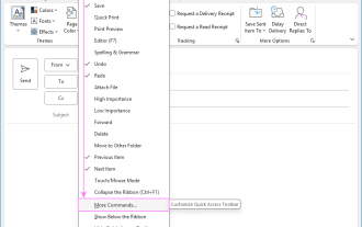
Jun 18, 2025 am 11:01 AM
This guide will walk you through how to customize, move, hide, and show the Quick Access Toolbar, helping you shape your Outlook workspace to fit your daily routine and preferences. The Quick Access Toolbar in Microsoft Outlook is a usefu
 Google Sheets IMPORTRANGE: The Complete Guide
Jun 18, 2025 am 09:54 AM
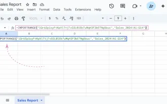
Google Sheets IMPORTRANGE: The Complete Guide
Jun 18, 2025 am 09:54 AM
Ever played the "just one quick copy-paste" game with Google Sheets... and lost an hour of your life? What starts as a simple data transfer quickly snowballs into a nightmare when working with dynamic information. Those "quick fixes&qu
 Don't Ignore the Power of F9 in Microsoft Excel
Jun 21, 2025 am 06:23 AM
Don't Ignore the Power of F9 in Microsoft Excel
Jun 21, 2025 am 06:23 AM
Quick LinksRecalculating Formulas in Manual Calculation ModeDebugging Complex FormulasMinimizing the Excel WindowMicrosoft Excel has so many keyboard shortcuts that it can sometimes be difficult to remember the most useful. One of the most overlooked
 6 Cool Right-Click Tricks in Microsoft Excel
Jun 24, 2025 am 12:55 AM
6 Cool Right-Click Tricks in Microsoft Excel
Jun 24, 2025 am 12:55 AM
Quick Links Copy, Move, and Link Cell Elements
 Prove Your Real-World Microsoft Excel Skills With the How-To Geek Test (Advanced)
Jun 17, 2025 pm 02:44 PM
Prove Your Real-World Microsoft Excel Skills With the How-To Geek Test (Advanced)
Jun 17, 2025 pm 02:44 PM
Whether you've recently taken a Microsoft Excel course or you want to verify that your knowledge of the program is current, try out the How-To Geek Advanced Excel Test and find out how well you do!This is the third in a three-part series. The first i
 How to recover unsaved Word document
Jun 27, 2025 am 11:36 AM
How to recover unsaved Word document
Jun 27, 2025 am 11:36 AM
1. Check the automatic recovery folder, open "Recover Unsaved Documents" in Word or enter the C:\Users\Users\Username\AppData\Roaming\Microsoft\Word path to find the .asd ending file; 2. Find temporary files or use OneDrive historical version, enter ~$ file name.docx in the original directory to see if it exists or log in to OneDrive to view the version history; 3. Use Windows' "Previous Versions" function or third-party tools such as Recuva and EaseUS to scan and restore and completely delete files. The above methods can improve the recovery success rate, but you need to operate as soon as possible and avoid writing new data. Automatic saving, regular saving or cloud use should be enabled
 5 New Microsoft Excel Features to Try in July 2025
Jul 02, 2025 am 03:02 AM
5 New Microsoft Excel Features to Try in July 2025
Jul 02, 2025 am 03:02 AM
Quick Links Let Copilot Determine Which Table to Manipu
