


Three practical functions for Excel data extraction and summary
Suppose you have a large workbook with beautifully formatted, filtered and sorted tables. You might think the work is done, but in reality, Excel is waiting for you to do more on these tables, eager to help you make the most of the hard work you have done so far.
This article will introduce three functions or combinations of functions that I often use that can be used to extract or summarize information in Excel tables.
VLOOKUP and HLOOKUP
VLOOKUP and HLOOKUP are both used to find and retrieve values ??at specific locations in a table.
- VLOOKUP relies on a vertical data table and looks up the first column (vertical) in the table.
- HLOOKUP relies on the horizontal data table and looks up the first row (horizontal) in the table.
VLOOKUP
Here, I have a list of test scores and the required grades for each grade (we call it Table 1). I also have a table with student grades (called Table 2 from this point). I want Excel to use the information in Table 1 to complete the missing columns in Table 2.

I will use VLOOKUP because I want Excel to look up the values ??in the first column of Table 1 to return the grades of each student in Table 2. The syntax of the VLOOKUP function is as follows:
<code>=VLOOKUP(a,b,c,d)</code>
Of:
- a is the value to be looked for (in the above example, that is the value in column E),
- b is a table containing the reference values ??(in this case, it is cells A1 to B9, or Table 1),
- c is the column number in that table (I want it to return the level, so it is the second column in Table 1), and
- d is an optional condition that tells Excel whether to approximate lookup values ??("TRUE") or exact lookup values ??("FALSE"). If left blank, the default value is TRUE.
So, in my case, I would enter this formula in cell F2 to calculate the grades of Tom and then use autofill to find other grades in the table:
<code>=VLOOKUP(E2,$A:$B,2,TRUE)</code>
I used the $ symbol to create an absolute reference for the above value b because I want Excel to continuously use cells A1 to B9 to find the value. I also used "TRUE" for the value d because the score boundary table contains ranges, not the rank assigned to a single score.

HLOOKUP
Here, we have the same level boundary information, but this time it is displayed horizontally. This means that the data we want to fetch is located in the second row of the boundary table.

The syntax of the HLOOKUP function is similar to that of VLOOKUP:
<code>=HLOOKUP(a,b,c,d)</code>
Of:
- a is the value to be found (in this example, the value in column C),
- b is an absolute reference to the cell containing the search value (in this case, it is A1 to I2),
- c is the row number in the table (I want it to return the level, so it is the second row), and
- d (optional) is "TRUE" (approximate value) or "FALSE" (exact value).
So I will enter this formula in cell C5 to calculate the grades of Tom and then use autofill to find other grades in the table:
<code>=VLOOKUP(a,b,c,d)</code>

INDEX and MATCH
Another effective way to find and retrieve values ??is through INDEX and MATCH, especially when used together. INDEX looks for and returns the value of the defined position, while MATCH looks for and returns the bit of the value. Together, they can implement dynamic data retrieval.
Single grammar
Before we look at these functions together, let's briefly view them individually.
The syntax of INDEX is
<code>=VLOOKUP(E2,$A:$B,2,TRUE)</code>
where a is the range of cells containing data, b is the row number to be evaluated, and c is the column number to be evaluated.
Based on this,
<code>=HLOOKUP(a,b,c,d)</code>
will evaluate cells B2 to D8 and return the values ??in the fourth row and second column in that range.
For MATCH, we follow
<code>=HLOOKUP(B5,$A:$I,2,TRUE)</code>
where x is the value we are looking for, y is the range of values ??we are looking for, and z (optional) is the matching type.
Based on this,
<code>INDEX(a,b,c)</code>
will tell me where the number 5 is in range B2 to B8, while 0 tells Excel to perform an exact match.
Use in combination
In this example, I want Excel to tell me the number of goals a specified player scores in a given month. More specifically, I want to know how many goals a player C scored in the third month, but I will create this formula so that I can change those conditions at any time.

To do this, I need Excel to determine the position of player C in the table and then tell me the value in the third column of the data.
In cell G4, I will start with the INDEX function because I want Excel to look up from my original data and return a value. I will then tell Excel where to look for that data.
<code>INDEX(B2:D8,4,2)</code>
The next part of the INDEX syntax is the line number, which will vary depending on the player I declare in cell G2. For example, if I want to find player A, it will be the first row. To do this, I'll start the MATCH function because I want Excel to match the player in cell G2 to the corresponding cell in player column (A2:A8) and figure out which row it is located. I also added the last 0 because I want Excel to return exact retrieval.
<code>=VLOOKUP(a,b,c,d)</code>
Now that I have told the Excel INDEX function line number, I need to do it with the column number. In my example, the column number represents the month number I typed in cell G3.
<code>=VLOOKUP(E2,$A:$B,2,TRUE)</code>
When I pressed the Enter key, Excel correctly told me that Player C had scored five goals in the third month.

Now I can change any value in my lookup table to find the total of any player in any month.

COUNTIF and SUMIF
As you can see from their names, these two functions count and sum values ??based on the conditions you set. Anything not included in your condition will not be added or counted, even if it is within the scope you specified.
COUNTIF
COUNTIF counts cells containing specific conditions. The syntax is
<code>=HLOOKUP(a,b,c,d)</code>
where a is the range you want to count, and b is the condition for counting.
Similarly, if I want to include multiple conditions, I will use COUNTIFS:
<code>=HLOOKUP(B5,$A:$I,2,TRUE)</code>
where a and b are the first range condition pairing, and c and d are the second range condition pairing ( You can have up to 127 pairs).
If any condition is a text or logical or mathematical symbol, it must be enclosed in double quotes.
In my salary table below, I want to calculate the number of people earning over £40,000 and the number of people who receive over £1,000 bonuses separately.

To calculate the number of employees who have a salary of more than £40,000, I need to enter this formula in cell D8:
<code>INDEX(a,b,c)</code>
where C2:C6 is the range of salary, ">40000" is the condition.
To calculate the number of service staff who receive over £1,000 bonus, I will use COUNTIFS because I have two conditions.
<code>INDEX(B2:D8,4,2)</code>
B2:B6,"Services" Part is the first range conditional pairing, D2:D6,">1000" is the second one.
Even if I separate thousands digits with commas in my table above, I don't include these commas in the formula, because commas have different functions here.

SUMIF
SUMIF sums cells according to the conditions you set. It works similarly to COUNTIF, but contains more parameters in parentheses. The syntax is
<code>MATCH(x,y,z)</code>
where a is the range of cells you want to evaluate before requesting, b is the condition for that evaluation (this can be a value or a cell reference), c (optional) is the cell to be added if it is different from a.
This time, we have to calculate three things: the total salary for more than £40,000, the total salary for the service department and the total bonus for employees who have more than £35,000.

First, to calculate the total salary of more than £40,000, I need to enter the following formula in cell D8:
<code>=VLOOKUP(a,b,c,d)</code>
where C2:C6 quotes the salary in the table, ">40000" tells Excel to sum only values ??exceeding this amount.
Next, I want to find out the total salary of the service department. So, in cell C9, I will type
<code>=VLOOKUP(E2,$A:$B,2,TRUE)</code>
where B2:B6 quotes department columns, "Services" Tell Excel I'm looking for employees in the service department, C2:C6 Tell Excel about these Employees' wages are summed.
My last task was to find out how much bonus the employees earning over £35,000 received. In cell C10, I will type
<code>=HLOOKUP(a,b,c,d)</code>
where C2:C6 tells Excel to evaluate wages, ">35000" are the conditions for these wages, D2:D6 Tell Excel to meet the conditions Personal bonus sum.

Excel also has the SUMIFS function, which performs the same procedure, but for multiple conditions. It is very different from SUMIF's syntax:
<code>=HLOOKUP(B5,$A:$I,2,TRUE)</code>
where a is the range of cells to be added, b is the first range to be evaluated, c is b, d and e are the next range condition pairing (you can have up to 127 pairs).
Using the table above, let's say I want to sum the bonuses for employees who earn more than £45,000. Here is the formula I will enter:
<code>INDEX(a,b,c)</code>
After mastering the above functions, try using the XLOOKUP function, which is designed to solve some of the disadvantages of VLOOKUP by finding the values ??on the left and right of the Find Value column without rearranging the data.
The above is the detailed content of My 3 Favorite Ways to Use Data in Excel Tables. For more information, please follow other related articles on the PHP Chinese website!

Hot AI Tools

Undress AI Tool
Undress images for free

Undresser.AI Undress
AI-powered app for creating realistic nude photos

AI Clothes Remover
Online AI tool for removing clothes from photos.

Clothoff.io
AI clothes remover

Video Face Swap
Swap faces in any video effortlessly with our completely free AI face swap tool!

Hot Article
Hot Tools

Notepad++7.3.1
Easy-to-use and free code editor

SublimeText3 Chinese version
Chinese version, very easy to use

Zend Studio 13.0.1
Powerful PHP integrated development environment

Dreamweaver CS6
Visual web development tools

SublimeText3 Mac version
God-level code editing software (SublimeText3)
Hot Topics


 How to Use Parentheses, Square Brackets, and Curly Braces in Microsoft Excel
Jun 19, 2025 am 03:03 AM
How to Use Parentheses, Square Brackets, and Curly Braces in Microsoft Excel
Jun 19, 2025 am 03:03 AM
Quick Links Parentheses: Controlling the Order of Opera
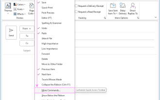 Outlook Quick Access Toolbar: customize, move, hide and show
Jun 18, 2025 am 11:01 AM
Outlook Quick Access Toolbar: customize, move, hide and show
Jun 18, 2025 am 11:01 AM
This guide will walk you through how to customize, move, hide, and show the Quick Access Toolbar, helping you shape your Outlook workspace to fit your daily routine and preferences. The Quick Access Toolbar in Microsoft Outlook is a usefu
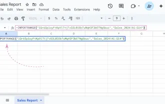 Google Sheets IMPORTRANGE: The Complete Guide
Jun 18, 2025 am 09:54 AM
Google Sheets IMPORTRANGE: The Complete Guide
Jun 18, 2025 am 09:54 AM
Ever played the "just one quick copy-paste" game with Google Sheets... and lost an hour of your life? What starts as a simple data transfer quickly snowballs into a nightmare when working with dynamic information. Those "quick fixes&qu
 Don't Ignore the Power of F9 in Microsoft Excel
Jun 21, 2025 am 06:23 AM
Don't Ignore the Power of F9 in Microsoft Excel
Jun 21, 2025 am 06:23 AM
Quick LinksRecalculating Formulas in Manual Calculation ModeDebugging Complex FormulasMinimizing the Excel WindowMicrosoft Excel has so many keyboard shortcuts that it can sometimes be difficult to remember the most useful. One of the most overlooked
 6 Cool Right-Click Tricks in Microsoft Excel
Jun 24, 2025 am 12:55 AM
6 Cool Right-Click Tricks in Microsoft Excel
Jun 24, 2025 am 12:55 AM
Quick Links Copy, Move, and Link Cell Elements
 How to recover unsaved Word document
Jun 27, 2025 am 11:36 AM
How to recover unsaved Word document
Jun 27, 2025 am 11:36 AM
1. Check the automatic recovery folder, open "Recover Unsaved Documents" in Word or enter the C:\Users\Users\Username\AppData\Roaming\Microsoft\Word path to find the .asd ending file; 2. Find temporary files or use OneDrive historical version, enter ~$ file name.docx in the original directory to see if it exists or log in to OneDrive to view the version history; 3. Use Windows' "Previous Versions" function or third-party tools such as Recuva and EaseUS to scan and restore and completely delete files. The above methods can improve the recovery success rate, but you need to operate as soon as possible and avoid writing new data. Automatic saving, regular saving or cloud use should be enabled
 5 New Microsoft Excel Features to Try in July 2025
Jul 02, 2025 am 03:02 AM
5 New Microsoft Excel Features to Try in July 2025
Jul 02, 2025 am 03:02 AM
Quick Links Let Copilot Determine Which Table to Manipu
 How to use Microsoft Teams?
Jul 02, 2025 pm 02:17 PM
How to use Microsoft Teams?
Jul 02, 2025 pm 02:17 PM
Microsoft Teams is not complicated to use, you can get started by mastering the basic operations. To create a team, you can click the "Team" tab → "Join or Create Team" → "Create Team", fill in the information and invite members; when you receive an invitation, click the link to join. To create a new team, you can choose to be public or private. To exit the team, you can right-click to select "Leave Team". Daily communication can be initiated on the "Chat" tab, click the phone icon to make voice or video calls, and the meeting can be initiated through the "Conference" button on the chat interface. The channel is used for classified discussions, supports file upload, multi-person collaboration and version control. It is recommended to place important information in the channel file tab for reference.
